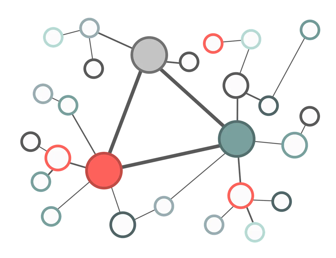
Unleashing the Power of Node Embedding: A Hands-on Example with Pytorch
"Graphs are a ubiquitous data structure"
In the beginning of my journey to let about graphs and applied machine learning on graph data I have come across this statement many times, however, it only made sense after applying graph algorithms to real-world problems and seeing how truly flexible and universal graph representation can be.
This is a first of many blog posts in a series of me attempting to learn and apply graph algorithms and sharing a summary of these learnings.
Introduction
Graphs represent a set of objects and the relationship among them. Taking for example financial systems, the nodes could represent a set of accounts and the edges could represent the transactions occurring among those accounts. If for example we are required to determine which accounts are fraudulent, we might want to explore the fact that fraud users behave similarly or might even be linked together forming a fraud network.
The corresponding edges could be represented in a table showing the source account, the destination account as well as any features associated with that edge. In this table below the amount is chosen as an example feature for each edge.
This is where the power of graphs really shines as it enables us to extract relationships in a way that enables us to train machine learning models to perform the required task.
Starting with an example
One of the first tasks using graphs is node classification, to do so we would like to create a node representation that could help in the classification task by summarising the node's structural features (i.e. It's location within the graph and how it is connected and influenced by its neighbours) as well as any additional features that we could have about the node itself.
This task is known as node representation learning, which is could also be viewed as creating node embedding from a given graph. In other words, we need a way to take the nodes in the graph and generate for each node a vector representing it.
Shallow embedding
The first class of algorithms used to create node embedding is known as shallow embedding, which is simply a learnable matrix that is used a lookup. Each row represents the learned embedding vector for a given node.
We can immediately realize the limitation of this approach as it can not generalize to unseen nodes and we can not use this matrix on new or dynamic graphs.
The main steps for learning such shallow embeddings are as follows:
- Initialize a matrix with NxM dimensions randomly, where N is the number of nodes and M is the chosen embedding dimension
- For each edge in the graph connecting nodes u and v calculate the dot product between the two vectors in the matrix representing their embeddings z_u \dot z_v
- Calculate a loss term to minimize the dot prod -log(dot_product)
- repeat till convergence
The main intuition behind this approach is that two connected nodes should have similar embedding vectors.
Shallow Embedding Pytorch Example
To demonstrate this approach, I will be using a dummy network generated NetworkX a popular graph processing package in Python
# import all relevant packages
import matplotlib.pyplot as plt
import networkx as nx
import numpy as np
import pandas as pd
import seaborn as sns
import torch
from sklearn.decomposition import PCA
from tqdm import tqdm

pd.set_option('display.max_columns', None)
pd.set_option('display.float_format', lambda x: '%.4f' % x)
EPS = 1e-15

# create a dummy barbell graph
graph = nx.barbell_graph(7, 3)

# visualize the graph
nx.draw_networkx(graph, label=True)
N = graph.number_of_nodes()
embedding_dim = 16

# define the shallow embedding matrix
embedding = torch.nn.Embedding(N, embedding_dim)

# define the optimizer
optimizer = torch.optim.Adam(list(embedding.parameters()), lr=0.01)

def train():
    """ Training loop """
    embedding.train()
    loss = 0

    # iterate over the edges in the graph
    # note that applying a for loop is very inefficient but easy to understand
    for (u, v) in graph.edges:
        z_u = embedding.weight[u]
        z_v = embedding.weight[v]

        # calculate the dot product
        out = (z_u * z_v).sum(dim=-1).view(-1)
        pos_loss = -torch.log(torch.sigmoid(out) + EPS).mean()
        loss += pos_loss
    loss.backward()
    optimizer.step()
    return loss.item()

for e in range(1, 101):
    loss = train()
    if e % 10 == 0:
        print(f"epoch: {e}, loss: {loss}")

@torch.no_grad()
def plot_embedding(embedding, title="PCA decomposition of the embeddings"):
    plt.figure()
    pca = PCA(n_components=2)
    z = pca.fit_transform(embedding.weight.numpy())
    sns.scatterplot(x=z[:, 0], y=z[:, 1], alpha=0.3, s=100)

    # show the label of each node on the figure
    for i, (x, y) in enumerate(z):
        plt.text(x, y, i)
    plt.title(title)

plot_embedding(embedding)
Conclusion
The provided code snippets creates a test graph (barbell) using networkX, then initializes the node embeddings and trains it using the dot product as a similarity metric between the nodes. The result shows that nodes that are connected together share a similar embedding values.
